
This article is inspired by the masterpiece of Gibbs Sampling tutorial by Resnik and Hardisty and also an awesome github repo by Bob Flagg. Both of these resources are excellent and highly recommended for anyone to read.
This article will show a step by step implementation of a Gibbs sampler for a Naive Bayes model in Python.
Let’s start with the problem definition. Assume that we would like to classify whether or not the sentiment of a document is either $0$ (negative) or $1$ (positive) visualized by the following image.

Moreover, the generative story of how the documents are generated as explained in $\S$2.1 of the paper is shown in the following image.
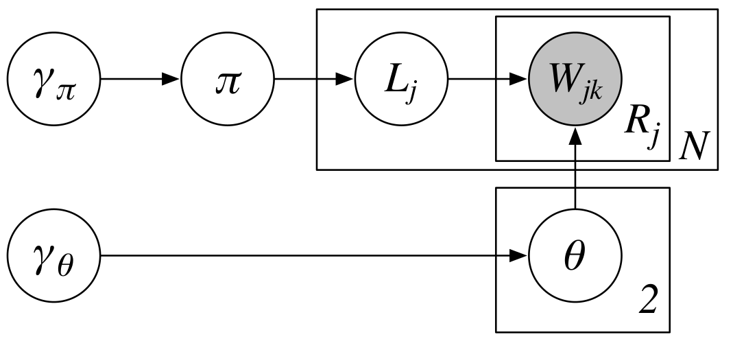
Let’s recall some of the notations from the paper. There are $6$ variables in the image and we shall discuss these variables one by one.
$\pmb{\gamma_\pi}$ is a vectorized version of hyperparameters from a Beta distribution. In the literature (Gelman et al., 2013), these hyperparameters usually are represented by $\alpha$ and $\beta$. In the paper, they are $\gamma_{\pi0}$ and $\gamma_{\pi1}$. Specifically, $\pmb{\gamma_\pi}$ is defined as follows:
\(\begin{equation}
\pmb{\gamma_\pi} = \begin{bmatrix} \gamma_{\pi0} \\ \gamma_{\pi1} \end{bmatrix}.
\end{equation} \tag{1}\label{eq:gamma-pi}\)
Secondly, $\pi$ is a random variable which has a Beta distribution, in other words
\[\begin{equation} \pi \sim \text{Beta}(\gamma_{\pi0}, \gamma_{\pi1}) \tag{2}\label{eq:beta}. \end{equation}\]Thirdly, $L_j$ is a random variable for $j$th document which has a Bernoulli distribution,
\[\begin{equation} L_j \sim \text{Bernoulli}(\pi) \tag{3}\label{eq:binomial}. \end{equation}\]Fourthly, $\pmb{\gamma_{\theta}}$ is a hyperparameter vector whose dimension is the size of vocabulary ($V$) and provided for a Dirichlet distribution. In the literature (Gelman et al., 2013), these hyperparameters usually are represented by $\alpha_1$, $\alpha_2$, $\ldots$, $\alpha_V$. In the paper, it is defined as a vector defined as follows:
\[\begin{equation} \pmb{\gamma_{\theta}} = \begin{bmatrix} \gamma_{\theta1} \\ \gamma_{\theta2} \\ \vdots \\ \gamma_{\theta V} \end{bmatrix} = \begin{bmatrix} 1 \\ 1 \\ \vdots \\ 1 \end{bmatrix} \tag{4}\label{eq:gamma-theta}. \end{equation}\]Fifthly, $\pmb{\theta}$ is a vector which contains two random variables, $\theta_0$ and $\theta_1$. Specifically, both $\theta_0$ and $\theta_1$ are Dirichlet distributions with $\pmb{\gamma_{\theta}}$ as their hyperparameters,
\[\begin{align} \theta_0 &\sim \text{Dirichlet}(\pmb{\gamma_{\theta}}) \tag{5}\label{eq:dirichlet-1}, \\ \theta_1 &\sim \text{Dirichlet}(\pmb{\gamma_{\theta}}) \tag{6}\label{eq:dirichlet-2}. \end{align}\]Last but not least, $\pmb{W}_j$ represents a probability distribution of $j$th document which modeled by a Multinomial distribution. As the $j$th document has $R_j$ words and probabilities of each word in the vocabulary, the Multinomial distribution is stated as follows:
\[\begin{equation} \pmb{W}_j \sim \text{Multinomial}(R_j, \theta_{L_j}), \text{ for }j = 1, \ldots, N. \tag{7}\label{eq:multinomial} \end{equation}\]Hopefully, now that we know what those variables are, we can move forward by programming them.
Let’s import all the libraries.
# import all the libraries
import numpy as np
from numpy.random import beta, binomial, dirichlet
Let’s define a function to sample labels for N documents with hyperparameter $\gamma_{\pi}$ (gamma_pi). The labels are either 0 (negative) or 1 (positive); additionally, the number of labels equal to the number of documents.
def sample_labels(N, gamma_pi):
    """Sample labels for N documents according to Beta distribution
    with a hyperparameter=gamma_pi

    Parameters
    ----------
    N        : int
               Number of documents
    gamma_pi : list with length=2
               Hyperparameters of the Beta distribution

    Returns
    -------
    array with shape (N,)
        Labels for the N documents
    """
    # pi is the Beta distribution with parameters gamma_pi[0] and gamma_pi[1]
    pi = beta(gamma_pi[0], gamma_pi[1])

    return binomial(1, pi, N)
Therefore, we have defined \(L_j\), for \(j=1,2, \ldots, N\) as in the graphical model.
Next, we implement how to generate documents. In generating documents, we employ Poisson distribution to determine the size of a document; in the paper, $R_j$ denotes the size of the $j$th document.
from numpy.random import multinomial, poisson

def generate_data(N, gamma_pi, gamma_theta, lmbda):
    """Generate N documents from a hyperparameter of binomial, Dirichlet, and Poisson

    Parameters
    ----------
    N           : int
                  Number of documents
    gamma_pi    : list with length=2
                  Hyperparameters of the Beta distribution
    gamma_theta : list with length=V with V denotes vocabulary size
                  Hyperparameters of the Dirichlet distribution
    lmbda       : int
                  Hyperparameter for Poisson distribution, denotes
                  number of words in a document
    Returns
    -------
    list of sets with shape (N,)
                  Each set represents a document which contains tuples (i,c)
                  with i denotes word index and c represents frequency of the word index i
    list of integer with shape (N,)
                  Labels of documents
    """
    # Sample N labels for N documents
    labels = sample_labels(N, gamma_pi)

    # Construct two Dirichlet distributions; each has gamma_theta as hyperparameters
    theta = dirichlet(gamma_theta, 2)

    # Initialize a list which contains N documents
    W = []
    for l in labels:
        R = poisson(lmbda)  # Sample a size of a document
        doc = multinomial(R, theta[l]) # Generate a document as a multinomial distribution
        # put the document into W
        # i = word index and c = frequency of the index i
        W.append({(i, c) for i,c in enumerate(doc) if c > 0})
    return W, labels
Basically, W contains N documents and each document consists of tuples and a tuple represents a word index and its frequency. For example, we have W as follows:
W = [{(0, 1), (1, 2), (2, 2), (3, 3), (4, 2)},
  {(0, 1), (1, 1), (2, 1), (3, 2), (4, 2)}]
This W represents $2$ documents. The first document contains word indices 0, 1, 2, 3, 4 with their frequencies 1, 2, 2, 3, 2 respectively. The second document contains word indices 0, 1, 2, 3, 4 with the frequencies 1, 1, 1, 2, 2 respectively.
Finally, we define initialize method as follows:
def initialize(W, labels, gamma_pi, gamma_theta):
    """Initialize all random variables and put them all into initial state

    Parameters
    ----------
    W           : list of sets
                  List of documents
    labels      : array with shape (N,)
                  Labels for the N documents
    gamma_pi    : list with length=2
                  Hyperparameters of the Beta distribution
    gamma_theta : list with length=V with V denotes vocabulary size
                  Hyperparameters of the Dirichlet distribution
    lmbda       : int
                  Hyperparameter for Poisson distribution, denotes
                  number of words in a document
    Returns
    -------
    A dictionary
                  A dictionary contains
                    C : an array with size (2,) that contains number of negative documents at index 0 and number of positive documents at index 1

                    N : an array with size (2, V) that contains frequencies of each word index in negative documents and frequencies of each word index in positive documents
    """
    # N is total number of documents
    N = len(W)

    # M is total number of labels which have been observed
    M = len(labels)

    # V is size of vocabulary
    V = len(gamma_theta)

    # Only sample the unobserved instances (N-M)
    L = sample_labels(N - M, gamma_pi)

    # Sample two Dirichlet distributions for each label (0 and 1)
    theta = dirichlet(gamma_theta, 2)

    # Initialize to record number of documents in each labels
    C = np.zeros((2,))

    # Add pseudcounts into observed evidence
    C += gamma_pi

    # Initialize cnts; cnts to record frequencies of word indices for each label
    cnts = np.zeros((2, V))

    # Add pseudcounts into observed evidence
    cnts += gamma_theta

    # Populate C and cnts
    for d, l in zip(W, labels.tolist() + L.tolist()):
        for i, c in d:
            cnts[l][i] += c
        C[l] += 1

    return {'C':C, 'N':cnts, 'L':L, 'theta':theta}
Variables C and cnts denotes \(\begin{bmatrix} C_0 + \gamma_{\pi 0} \\ C_1 + \gamma_{\pi 1} \end{bmatrix}\) and \(\begin{bmatrix}
\pmb{\mathcal{N}_{\mathbb{C}_0}} + \pmb{\gamma_{\theta 0}} \\
\pmb{\mathcal{N}_{\mathbb{C}_1}} + \pmb{\gamma_{\theta 1}}
\end{bmatrix}\) in the paper respectively. Particularly, \(\pmb{\mathcal{N}_{\mathbb{C}_0}}\), \(\pmb{\mathcal{N}_{\mathbb{C}_1}}\), \(\pmb{\gamma_{\theta 0}}\), and \(\pmb{\gamma_{\theta 1}}\) are vectors with the size \(1 \times V\).
We have reached the end of the first part of Gibbs Sampling for the Uninitiated part 1. In part 2, we shall discuss the building of Gibbs sampler, specifically, how to implement Equation ($49$) on page $16$ of the paper:
\[\begin{equation} \text{Pr(L}_j = x | \mathbf{L}^{(-j)}, \mathbb{C}^{(-j)}, \mathbf{\theta_0}, \mathbf{\theta_1}; \mathbf{\mu}) = \frac{C_x + \gamma_{\pi x} - 1}{N + \gamma_{\pi 1} + \gamma_{\pi 0} - 1} \prod_{i=1}^{V}{\theta_{x,i}^{\text{W}_{ji}}}.\tag{8}\label{eq:update-equation} \end{equation}\]The playground of this tutorial is also provided as Jupyter notebook in this repo.