
[EN] Variance and Covariance of Categorical Distribution
Published:
This post is inspired by the lecture given by David Blei on Thursday, 17 September 2020. One of the topics he explained was related to a categorical variable and a categorical distribution. This post will elaborate those two concepts. Let’s get started.
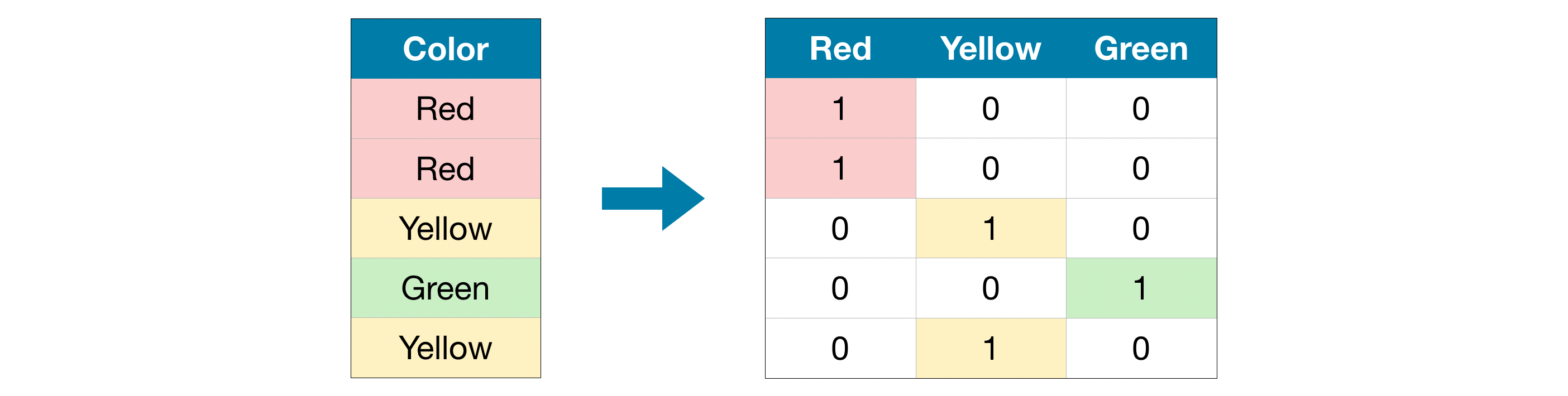 \( \pmb{\text{Figure 1}} \) : A categorical variable ( \( \text{Color} \)) and its values ( \( \text{Red} \), \( \text{Yellow} \), and \( \text{Green} \) ). Image taken from Kaggle, some rights reserved.
\(\text{Figure 1}\) shows an example of categorical values stored in a categorical variable, \(\text{Color}\). Basically, a categorical variable takes one of \(K\) values and each categorical value is represented by a \(K\)-vector with a single \(1\) and otherwise \(0\)s.
Let’s denote a categorical variable as \(x^{(k)}\) which means that the \(k\)th component of it has a a single \(1\) and otherwise \(0\)s.
For example, the categorical variable in \(\text{Figure 1}\) has \(3\) values ( \(\text{Red}\), \(\text{Yellow}\), and \(\text{Green}\) ) and each value is represented by \(3\)-vector with a single \(1\) and otherwise \(0\)s as follows:
\[\begin{align} \text{Red} &= x^{(1)} = (1, 0, 0 ) \\ \text{Yellow} &= x^{(2)} = (0, 1, 0 ) \tag{1}\label{eq:yellow} \\ \text{Green} &= x^{(3)} = (0, 0, 1 ). \end{align}\]The \(K\)-vector with single \(1\) and otherwise \(0\)s is commonly named one-hot vector.
A categorical distribution is parameterized by \(\theta\). Moreover, \(\pmb{\theta}\) specifies the probability of each categorical value. Suppose we have \(K\) categorical values; therefore,
\[\begin{equation} \theta = (\theta_1, \theta_2, \ldots, \theta_K) \tag{2}\label{eq:theta} \end{equation}\]with
\[\begin{equation} \sum_{k=1}^{K}{\theta_k} = 1 \text{ and } 0 \leq \theta_k \leq 1 \text{ for }k=1, \ldots, K. \tag{3}\label{eq:theta-constraints} \end{equation}\]Consider that \(X^{(k)}\) is a random categorical variable which takes one of \(K\) values. Moreover, since \(X^{(k)}\) is random variable, it has categorical distribution that is described by a discrete probability distribution,
\(\begin{equation} \text{p}(x^{(k)}) = \prod_{l=1}^{K}{\theta_{l}^{x^{(l)}}} \tag{4}\label{eq:pdf-categorical} \end{equation}\)
with \(x^{(l)}\) is the \(l\)th component of \(x^{(k)}\). Additionally, we elaborate Equation \eqref{eq:pdf-categorical} into
Let’s put Equation \eqref{eq:pdf-categorical-simplified} into practice and demonstrate it in one example. Suppose we want to compute \(\text{p}(\text{Yellow})\) in Equation \eqref{eq:yellow},
\[\begin{align} \text{p}(\text{Yellow}) &= \text{p}(x^{(2)}) \\ &= \text{p}((0,1,0)) & \Rightarrow \text{1st} = 0, \text{2nd} = 1, \text{3rd} = 0 \\ &= \prod_{l=1}^{3}{\theta_{l}^{x^{(l)}}} \\ &= \theta_{1}^{x^{(1)}} \times \theta_{2}^{x^{(2)}} \times \theta_{3}^{x^{(3)}} \\ &= \theta_{1}^{0} \times \theta_{2}^{1} \times \theta_{3}^{0} \\ &= \theta_{2}. \end{align}\]With Equation \eqref{eq:pdf-categorical-simplified} in hand, we are now ready to compute the expectation of \(X^{(k)}\) as
\[\begin{align} \text{E}(X^{(k)}) &= \sum_{l=1}^{K}{x^{(l)} \text{p}(x^{(l)})} \\ &= \underbrace{0 \times \text{p}(x^{(1)})}_{1\text{st}} + \underbrace{0 \times \text{p}(x^{(2)})}_{2\text{nd}} + \cdots + \underbrace{1 \times \text{p}(x^{(k)})}_{k\text{th}} + \cdots + \underbrace{0 \times \text{p}(x^{(K)}}_{K\text{th}}) \\ &= \text{p}(x^{(k)}) \\ &= \theta_k. \tag{6}\label{eq:expectation} \end{align}\]Next, we compute the Variance, \(\text{Var}\), as follows:
\[\begin{align} \text{Var}(X^{(k)}) &= \underbrace{\text{E}((X^{(k)})^2)}_{\text{Part I}} - \underbrace{(\text{E}(X^{(k)}))^2}_{\text{Part II}}. & \text{the definition of variance} \tag{7}\label{eq:variance-definition} \\ \end{align}\]Next, we compute \(\text{Part I}\), \(\text{E}((X^{(k)})^2)\), as follows:
\[\begin{align} \text{E}((X^{(k)})^2) &= \sum_{l=1}^{K}{(x^{(l))^2} \text{p}(x^{(l)})} \\ &= \underbrace{0^2 \times \text{p}(x^{(1)})}_{1\text{st}} + \underbrace{0^2 \times \text{p}(x^{(2)})}_{2\text{nd}} + \cdots + \underbrace{1^2 \times \text{p}(x^{(k)})}_{k\text{th}} + \cdots + \underbrace{0^2 \times \text{p}(x^{(K)}}_{K\text{th}}) \\ &= \text{p}(x^{(k)}) \\ &= \theta_k. \tag{8}\label{eq:expectation-x-square} \end{align}\]Now, we can finalize computing the Variance in Equation \eqref{eq:variance-definition},
\[\begin{align} \text{Var}(X^{(k)}) &= \text{E}((X^{(k)})^2) - (\text{E}(X^{(k)}))^2 && \text{by definition of variance} \\ &= \theta_k - (\theta_k)^2 && \text{using Equation }\eqref{eq:expectation} \text{ and }\eqref{eq:expectation-x-square} \\ &= \theta_k (1 - \theta_k). && \text{using distributive property} \tag{9}\label{eq:variance} \end{align}\]Last but not least, we shall compute the Covariance, \(\text{Cov}(X^{(j)}, X^{(k)})\). We start by the definition of Covariance,
\[\begin{align} \text{Cov}(X^{(j)}, X^{(k)}) &= \underbrace{\text{E}(X^{(j)} X^{(k)})}_{\text{Part I}} - \underbrace{(\text{E}(X^{(j)}) E(X^{(k)}))}_{\text{Part II}}. && \text{by definition} \tag{10}\label{eq:covariance} \end{align}\]Let’s compute the \(\text{Part I}\) as follows:
\[\begin{align} \text{E}(X^{(j)} X^{(k)}) &= (0)(0) \theta_1 + \cdots + \underbrace{(1)(0) \theta_j}_{j\text{th}} + \cdots + \underbrace{(0)(1) \theta_k}_{k\text{th}} + \cdots + (0)(0) \theta_K \\ &= 0. \tag{11}\label{eq:covariance-zero} \end{align}\]Eventually, we can finalize Equation \eqref{eq:covariance} as
\[\begin{align} \text{Cov}(X^{(j)}, X^{(k)}) &= \text{E}(X^{(j)} X^{(k)}) - (\text{E}(X^{(j)}) E(X^{(k)})) \\ &= 0 - \theta_j \theta_k && \text{using Equation } \eqref{eq:expectation} \text{ and }\eqref{eq:covariance-zero} \\ &= - \theta_j \theta_k. \end{align}\]To conclude, we have shown how to derive the expectation, variance, and covariance of a categorical distribution. We hope this post helps anyone who wants to understand a categorical distribution.