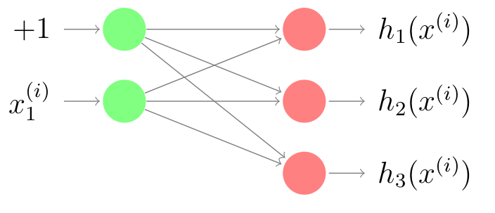
This article attempts to find gradients of a softmax output layer. This knowledge proves useful when we want to utilize backpropagation algorithm to compute gradients of neural networks with a softmax output layer. Furthermore, page 3 from the outstanding Notes on Backpropagation by Peter Sadowski has inspired this article a lot.

Suppose that we have a multiclass classification problem with 3 (three) choices that are label $1$, label $2$, and label $3$. The image below shows the very simple artificial neural networks with two layers; particulary, we set the output layer as a softmax output layer.

Concretely, we utilize one-hot encoding for the three choices as follows:

\(\begin{bmatrix} 1 \\ 0 \\ 0 \end{bmatrix}\), \(\begin{bmatrix} 0 \\ 1 \\ 0 \end{bmatrix}\), and \(\begin{bmatrix} 0 \\ 0 \\ 1 \end{bmatrix}\) are the representations for label $1$, label $2$, and label $3$ respectively.

Let us define our dataset, \(X = \{ (x^{(1)}, y^{(1)}), (x^{(2)}, y^{(2)}), \ldots, (x^{(m)}, y^{(m)}) \}\), which has \(m\) instances and

\[\begin{equation} x^{(i)} = \begin{bmatrix} 1 \\ x_1^{(i)} \end{bmatrix} \text{ and } y^{(i)} = \begin{bmatrix} y_1^{(i)} \\ y_2^{(i)} \\ y_3^{(i)} \end{bmatrix} \end{equation}\tag{1}\label{eq:label-y}\]

with \(y_1^{(i)}\), \(y_2^{(i)}\), \(y_3^{(i)}\) have only binary values (either 0 or 1) for \(i = 1, 2, \ldots, m\).

We employ softmax functions as our predictions. Specifically, we define our first hypoteses

\[\begin{equation} h_1(x^{(i)}) = \frac{\exp{(\Theta_{10} + \Theta_{11} x_1^{(i)}})}{\exp{(\Theta_{10} + \Theta_{11} x_1^{(i)})}+\exp{(\Theta_{20} + \Theta_{21} x_1^{(i)})}+\exp{(\Theta_{30} + \Theta_{31} x_1^{(i)}})} \end{equation}\tag{2}\label{eq:hyphotesis-1}\]

the second hyphotesis,

\[\begin{equation} h_2(x^{(i)}) = \frac{\exp{(\Theta_{20} + \Theta_{21} x_1^{(i)})}}{\exp{(\Theta_{10} + \Theta_{11} x_1^{(i)})}+\exp{(\Theta_{20} + \Theta_{21} x_1^{(i)})}+\exp{(\Theta_{30} + \Theta_{31} x_1^{(i)}})} \end{equation}\tag{3}\label{eq:hyphotesis-2}\]

the third hyphotesis,

\[\begin{equation} h_3(x^{(i)}) = \frac{\exp{(\Theta_{30} + \Theta_{31} x_1^{(i)})}}{\exp{(\Theta_{10} + \Theta_{11} x_1^{(i)})}+\exp{(\Theta_{20} + \Theta_{21} x_1^{(i)})}+\exp{(\Theta_{30} + \Theta_{31} x_1^{(i)}})} \end{equation}\tag{4}\label{eq:hyphotesis-4}\]

and the cost function,

\[\begin{equation} J(\Theta) = - \sum_{i=1}^{m} ( y_1^{(i)} \log h_1(x^{(i)}) + y_2^{(i)} \log h_2(x^{(i)}) + y_3^{(i)} \log h_3(x^{(i)}) ) \end{equation}\tag{5}\label{eq:cost-function}\]

with

\[\begin{equation} \Theta = \begin{bmatrix} \Theta_{10} & \Theta_{11} \\ \Theta_{20} & \Theta_{21} \\ \Theta_{30} & \Theta_{31} \end{bmatrix}. \end{equation}\tag{6}\label{eq:the-theta}\]

Now we will show how to derive the gradient for these softmax activation function. In other words,

What are \(\frac{\partial J}{\partial \Theta_{10}}\), \(\frac{\partial J}{\partial \Theta_{11}}\), \(\frac{\partial J}{\partial \Theta_{20}}\), \(\frac{\partial J}{\partial \Theta_{21}}\), \(\frac{\partial J}{\partial \Theta_{30}}\), and \(\frac{\partial J}{\partial \Theta_{31}}\)?

Firstly, We show how to derive \(\frac{\partial J}{\partial \Theta_{10}}\) and \(\frac{\partial J}{\partial \Theta_{11}}\).

Let’s derive \(\frac{\pmb{\partial J}}{\pmb{\partial \Theta_{10}}}\)

By employing Multivariable Calculus, we obtain

\[\begin{equation} \frac{\partial J}{\partial \Theta_{10}} = \underbrace{\frac{\partial J}{\partial h_1}\frac{\partial h_1}{\partial \Theta_{10}}}_{\text{Part I}} + \underbrace{\frac{\partial J}{\partial h_2}\frac{\partial h_2}{\partial \Theta_{10}}}_{\text{Part II}} + \underbrace{\frac{\partial J}{\partial h_3}\frac{\partial h_3}{\partial \Theta_{10}}}_{\text{Part III}}. \end{equation}\tag{7}\label{eq:gradient-10}\]

The Part I consists of \(\frac{\partial J}{\partial h_1}\frac{\partial h_1}{\partial \Theta_{10}}\). Specifically,

\[\begin{equation} \frac{\partial J}{\partial h_1} = - \sum_{i=1}^{m}{\frac{y_1^{(i)}}{h_1(x^{(i)})}}. \end{equation}\tag{8}\label{eq:gradient-10-1}\]

By defining

\[\begin{equation} u = \exp{(\Theta_{10} + \Theta_{11}x_1^{(i)})} \end{equation}\tag{9}\label{eq:gradient-10-2}\]

and

\[\begin{equation} v = \exp{(\Theta_{10} + \Theta_{11}x_1^{(i)})} + \exp{(\Theta_{20} + \Theta_{21}x_1^{(i)})} + \exp{(\Theta_{30} + \Theta_{31}x_1^{(i)})} \end{equation}\tag{10}\label{eq:gradient-10-3}\]

and Quotient Rule, we are able to compute \(\frac{\partial h_1}{\partial \Theta_{10}}\) as follows:

\[\begin{align} \frac{\partial h_1}{\partial \Theta_{10}} &= \frac{u^{\prime} v - u v^{\prime}}{v^2} \\ &= \frac{(\exp{(\Theta_{10} + \Theta_{11}x_1^{(i)})})(\exp{(\Theta_{10} + \Theta_{11}x_1^{(i)})} + \exp{(\Theta_{20} + \Theta_{21}x_1^{(i)})} + \exp{(\Theta_{30} + \Theta_{31}x_1^{(i)})}) - (\exp{(\Theta_{10} + \Theta_{11}x_1^{(i)})})^2}{(\exp{(\Theta_{10} + \Theta_{11}x_1^{(i)})} + \exp{(\Theta_{20} + \Theta_{21}x_1^{(i)})} + \exp{(\Theta_{30} + \Theta_{31}x_1^{(i)})})^2} \\ &= \frac{\exp{(\Theta_{10} + \Theta_{11}x_1^{(i)})}}{\exp{(\Theta_{10} + \Theta_{11}x_1^{(i)})} + \exp{(\Theta_{20} + \Theta_{21}x_1^{(i)})} + \exp{(\Theta_{30} + \Theta_{31}x_1^{(i)})}} - \left( \frac{\exp{(\Theta_{10} + \Theta_{11}x_1^{(i)})}}{\exp{(\Theta_{10} + \Theta_{11}x_1^{(i)})} + \exp{(\Theta_{20} + \Theta_{21}x_1^{(i)})} + \exp{(\Theta_{30} + \Theta_{31}x_1^{(i)})}} \right)^2 \\ &= h_1(x^{(i)}) - (h_1(x^{(i)}))^2 \\ &= h_1(x^{(i)}) (1 - h_1(x^{(i)}))\tag{11}\label{eq:gradient-10-4} \end{align}\]

Finally, we can compute \(\frac{\partial J}{\partial h_1}\frac{\partial h_1}{\partial \Theta_{10}}\) by combining Equation \eqref{eq:gradient-10-1} and Equation \eqref{eq:gradient-10-4} as follows:

\[\require{cancel} \begin{align} \frac{\partial J}{\partial h_1}\frac{\partial h_1}{\partial \Theta_{10}} &= - \sum_{i=1}^{m}{\frac{y_1^{(i)}}{\cancel{h_1(x^{(i)})}} \cancel{h_1(x^{(i)})} (1 - h_1(x^{(i)}) )} \\ &= - \sum_{i=1}^{m}{y_1^{(i)} (1 - h_1(x^{(i)}))}\tag{12}\label{eq:gradient-10-5} \end{align}\]

The Part II consists of \(\frac{\partial J}{\partial h_2}\frac{\partial h_2}{\partial \Theta_{10}}\). Specifically,

\[\begin{equation} \frac{\partial J}{\partial h_2} = - \sum_{i=1}^{m}{\frac{y_2^{(i)}}{h_2(x^{(i)})}}. \end{equation}\tag{13}\label{eq:gradient-10-6}\]

Again, by defining

\[\begin{equation} u = \exp{(\Theta_{20} + \Theta_{21}x_1^{(i)})} \end{equation},\tag{14}\label{eq:gradient-10-7}\]

using Equation \eqref{eq:gradient-10-3}, and Quotient Rule, we can compute \(\frac{\partial h_2}{\partial \Theta_{10}}\)

\[\begin{align} \frac{\partial h_2}{\partial \Theta_{10}} &= \frac{u^{\prime} v - u v^{\prime}}{v^2} \\ &= \frac{0 - \exp{(\Theta_{20} + \Theta_{21} x_1^{(i)})} \exp{(\Theta_{10} + \Theta_{11} x_1^{(i)})}}{(\exp{(\Theta_{10} + \Theta_{11}x_1^{(i)})} + \exp{(\Theta_{20} + \Theta_{21}x_1^{(i)})} + \exp{(\Theta_{30} + \Theta_{31}x_1^{(i)})})^2} \\ &= - \left(\frac{\exp{(\Theta_{20} + \Theta_{21} x_1^{(i)})}}{\exp{(\Theta_{10} + \Theta_{11}x_1^{(i)})} + \exp{(\Theta_{20} + \Theta_{21}x_1^{(i)})} + \exp{(\Theta_{30} + \Theta_{31}x_1^{(i)})}} \right) \left( \frac{\exp{(\Theta_{10} + \Theta_{11} x_1^{(i)})}}{\exp{(\Theta_{10} + \Theta_{11}x_1^{(i)})} + \exp{(\Theta_{20} + \Theta_{21}x_1^{(i)})} + \exp{(\Theta_{30} + \Theta_{31}x_1^{(i)})}} \right) \\ &= - h_2(x^{(i)}) h_1(x^{(i)}) \tag{15}\label{eq:gradient-10-8} \end{align}\]

By using Equation \eqref{eq:gradient-10-6} and Equation \eqref{eq:gradient-10-8}, \(\frac{\partial J}{\partial h_2}\frac{\partial h_2}{\partial \Theta_{10}}\) can be computed as

\[\begin{align} \frac{\partial J}{\partial h_2}\frac{\partial h_2}{\partial \Theta_{10}} &= + \sum_{i=1}^{m}{\frac{y_2^{(i)}}{\cancel{h_2(x^{(i)})}} \cancel{h_2(x^{(i)})} h_1(x^{(i)})} \\ &= \sum_{i=1}^{m}{y_2^{(i)} h_1(x^{(i)})}.\tag{16}\label{eq:gradient-10-9} \end{align}\]

Lastly, the Part III consists of \(\frac{\partial J}{\partial h_3}\frac{\partial h_3}{\partial \Theta_{10}}\).

Particularly,

\[\begin{equation} \frac{\partial J}{\partial h_3} = - \sum_{i=1}^{m}{\frac{y_3^{(i)}}{h_3(x^{(i)})}}. \end{equation}\tag{17}\label{eq:gradient-10-10}\]

Again, by defining

\[\begin{equation} u = \exp{(\Theta_{30} + \Theta_{31}x_1^{(i)})} \end{equation},\tag{18}\label{eq:gradient-10-11}\]

using Equation \eqref{eq:gradient-10-3}, and Quotient Rule, we can compute \(\frac{\partial h_3}{\partial \Theta_{10}}\)

\[\begin{align} \frac{\partial h_3}{\partial \Theta_{10}} &= \frac{u^{\prime} v - u v^{\prime}}{v^2} \\ &= \frac{0 - \exp{(\Theta_{30} + \Theta_{31} x_1^{(i)})} \exp{(\Theta_{10} + \Theta_{11} x_1^{(i)})}}{(\exp{(\Theta_{10} + \Theta_{11}x_1^{(i)})} + \exp{(\Theta_{20} + \Theta_{21}x_1^{(i)})} + \exp{(\Theta_{30} + \Theta_{31}x_1^{(i)})})^2} \\ &= - \left(\frac{\exp{(\Theta_{30} + \Theta_{31} x_1^{(i)})}}{\exp{(\Theta_{10} + \Theta_{11}x_1^{(i)})} + \exp{(\Theta_{20} + \Theta_{21}x_1^{(i)})} + \exp{(\Theta_{30} + \Theta_{31}x_1^{(i)})}} \right) \left( \frac{\exp{(\Theta_{10} + \Theta_{11} x_1^{(i)})}}{\exp{(\Theta_{10} + \Theta_{11}x_1^{(i)})} + \exp{(\Theta_{20} + \Theta_{21}x_1^{(i)})} + \exp{(\Theta_{30} + \Theta_{31}x_1^{(i)})}} \right) \\ &= - h_3(x^{(i)}) h_1(x^{(i)}) \tag{19}\label{eq:gradient-10-12} \end{align}\]

Again by using Equation \eqref{eq:gradient-10-10} and Equation \eqref{eq:gradient-10-12}, \(\frac{\partial J}{\partial h_3}\frac{\partial h_3}{\partial \Theta_{10}}\) can be computed as

\[\begin{align} \frac{\partial J}{\partial h_3}\frac{\partial h_3}{\partial \Theta_{10}} &= + \sum_{i=1}^{m}{\frac{y_3^{(i)}}{\cancel{h_3(x^{(i)})}} \cancel{h_3(x^{(i)})} h_1(x^{(i)})} \\ &= \sum_{i=1}^{m}{y_3^{(i)} h_1(x^{(i)})}.\tag{20}\label{eq:gradient-10-13} \end{align}\]

Finally, combining Equation \eqref{eq:gradient-10-5}, \eqref{eq:gradient-10-9}, and \eqref{eq:gradient-10-13} we obtain

\[\begin{align} \frac{\partial J}{\partial \Theta_{10}} &= \frac{\partial J}{\partial h_1}\frac{\partial h_1}{\partial \Theta_{10}} + \frac{\partial J}{\partial h_2}\frac{\partial h_2}{\partial \Theta_{10}} + \frac{\partial J}{\partial h_3}\frac{\partial h_3}{\partial \Theta_{10}} \\ &= \sum_{i=1}^{m}{\left( -y_1^{(i)} + y_1^{(i)} h_1(x^{(i)}) + y_2^{(i)} h_1(x^{(i)}) + y_3^{(i)} h_1(x^{(i)}) \right)} \\ &= \sum_{i=1}^{m}{\left( -y_1^{(i)} + h_1(x^{(i)}) \underbrace{(y_1^{(i)} + y_2^{(i)} + y_3^{(i)})}_{\text{equals to }1} \right)} \\ &= \sum_{i=1}^{m}{(h_1(x^{(i)}) - y_1^{(i)})}\tag{21}\label{eq:final-gradient-1} \end{align}\]

With the same technique, we also obtain \(\begin{equation} \frac{\partial J}{\partial \Theta_{11}} = \sum_{i=1}^{m}{( h_1(x^{(i)}) - y_1^{(i)} ) x_1^{(i)}} \end{equation}\tag{22}\label{eq:final-gradient-2}\)

or in general form,

\[\begin{equation} \frac{\partial J}{\partial \Theta_{kj}} = \sum_{i=1}^{m}{( h_k(x^{(i)}) - y_k^{(i)} ) x_j^{(i)}} \end{equation}\tag{23}\label{eq:final-gradient-3}\]

with \(x_j^{(i)} = 0\) if \(j = 0\). Although the calculation in output layer is different, surprisingly, Equation \eqref{eq:final-gradient-3} is similar to gradients of sigmoid output layer. Hence, utilizing softmax output layer should be no worries.