
This post is the continuation of the post which derives a predictive distribution from Poisson & Gamma Conjugate Pair.

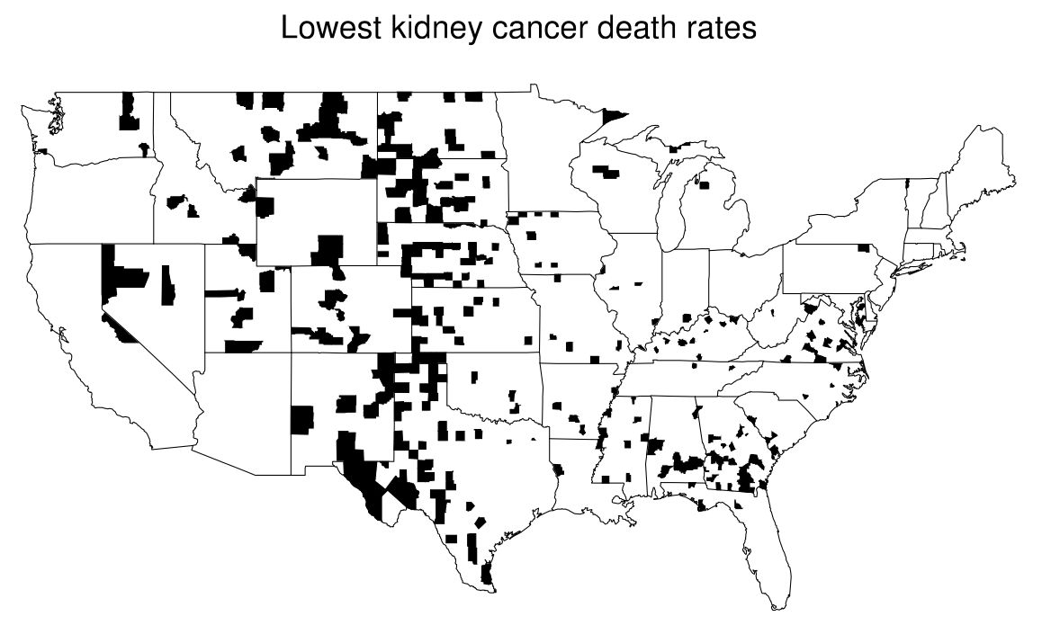
Previously, $\text{Figure 1}$ shows misleading patterns in the maps of cancer death rates which are modeled by a posterior distribution, in this case a Gamma distribution. The likelihood is defined as
\[\begin{equation} y_j \mid \theta \sim \text{Poisson}(10 n_j \theta_j), \tag{1}\label{eq:likelihood} \end{equation}\]the prior distribution is
\[\begin{equation} \theta_j \sim \text{Gamma}(\alpha, \beta). \tag{2}\label{eq:prior} \end{equation}\]Calculating the posterior distribution by multiplying Equation \eqref{eq:likelihood} and \eqref{eq:prior}, we arrive at
\[\begin{equation} \theta_j \mid y_j \sim \text{Gamma}(\alpha + y_j, \beta + 10 \, n_j). \tag{3}\label{eq:posterior} \end{equation}\]The previous post shows that
\[\begin{equation} \Pr(y_j) = \int \Pr(y_j \mid \theta_j) \Pr(\theta_j) \, d\theta \tag{4}\label{eq:predictive-distribution} \end{equation}\]is a negative binomial distribution, $\text{Neg-bin}( \alpha, \frac{\beta}{10 n_j} )$.
This post attempts to show the mean ($\text{E}(y_j)$) and variance ($\text{var}(y_j)$) of a negative binomial distribution.
Specifically, we utilize the following two equations,
\[\begin{equation} \text{E}(u) = \text{E}(\text{E}( u \mid v )) \tag{5}\label{eq:conditional-mean} \end{equation}\]and
\[\begin{equation} \text{var}(u) = \text{E}(\text{var}(u \mid v)) + \text{var}(\text{E}(u \mid v)) \tag{6}\label{eq:conditional-variance} \end{equation}\]in our attempt.
Firstly, we employ Equation \eqref{eq:conditional-mean} to find $\text{E}(y_j)$ as follows:
\[\begin{align} \text{E}(y_j) &= \iint y_j \Pr(y_j, \theta_j) \, dy_j \, d\theta_j && \text{definition of expectation} \tag{7}\label{eq:definition-expectation} \\ &= \iint y_j \Pr(y_j \mid \theta_j) \Pr(\theta_j) \, dy_j \, d\theta_j && \text{definition of conditional probability} \tag{8}\label{eq:definition-conditional-prob} \\ &= \iint y_j \Pr(y_j \mid \theta_j) \, dy_j \Pr(\theta_j) \, d\theta_j && \text{just rearranging} \tag{9}\label{eq:rearranging} \\ &= \int \underbrace{\int y_j \Pr(y_j \mid \theta_j) \, dy_j}_{\text{An expectation}} \Pr(\theta_j) \, d\theta_j && \tag{10}\label{eq:an-expectation} \\ &= \int \text{E}(y_j \mid \theta_j) \Pr(\theta_j) \, d\theta_j. \tag{11}\label{eq:gathering-expectation} \end{align}\]Recall that $y_j \mid \theta_j$ has $\text{Poisson}(10 n_j \theta_j)$ based on Equation \eqref{eq:likelihood}; therefore, we can proceed from Equation \eqref{eq:gathering-expectation} as follows:
\[\begin{align} \text{E}(y_j) &= \int 10 n_j \theta_j \Pr(\theta_j) \, d\theta_j && \text{because }\text{E}(y_j \mid \theta_j) = 10 n_j \theta_j \tag{12}\label{eq:inserting-expectation} \\ &= \int 10 n_j \theta_j \frac{\beta^\alpha}{\Gamma (\alpha)} \theta_j^{\alpha-1} e^{-\beta \theta_j} \, d\theta_j && \text{based on Equation }\eqref{eq:prior}, \text{a Gamma} \tag{13}\label{eq:inserting-gamma} \\ &= \int 10 n_j \frac{\beta^\alpha}{\Gamma (\alpha)} \theta_j^{\alpha} e^{-\beta \theta_j} \, d\theta_j && \text{adding }\theta_j \text{ into }\theta_j^{\alpha-1} \tag{14}\label{eq:mean-1} \\ &= 10 n_j \frac{\beta^\alpha}{\Gamma(\alpha)} \int \theta_j^{(\alpha+1)-1} e^{-\beta \theta_j} \, d\theta_j && \text{getting out }10 n_j \frac{\beta^\alpha}{\Gamma(\alpha)} \tag{15}\label{eq:mean-2} \end{align}\]Remember that if we have
\[\begin{equation} \theta_j \sim \text{Gamma}(\alpha, \beta) \tag{16}\label{eq:gamma-dist} \end{equation}\]then, the integral of probability density function of $\theta_j$ over $[0, \infty]$ is $1$,
\[\begin{align} \int_{0}^{\infty} \frac{\beta^{\alpha+1}}{\Gamma(\alpha+1)} \theta_j^{(\alpha+1)-1} e^{-\beta \theta_j} \, d\theta_j = 1 &\Longleftrightarrow \int_{0}^{\infty} \theta_j^{(\alpha+1)-1} e^{-\beta \theta_j} \, d\theta_j = \frac{\Gamma(\alpha+1)}{\beta^{\alpha+1}}. \tag{17}\label{eq:gamma-dist-1} \end{align}\]Substituting Equation \eqref{eq:gamma-dist-1} into Equation \eqref{eq:mean-2}, we have the mean of negative binomial distribution:
\[\require{cancel} \begin{align} \text{E}(y_j) &= 10 n_j \frac{\beta^\alpha}{\Gamma(\alpha)} \frac{\Gamma(\alpha+1)}{\beta^{\alpha+1}} \\ &= 10 n_j \frac{\cancel{\beta^\alpha}}{\Gamma(\alpha)} \frac{\Gamma(\alpha+1)}{\cancel{\beta^\alpha}\beta} \\ &= 10 n_j \frac{\alpha !}{(\alpha - 1)!} \frac{1}{\beta} && \text{because }\Gamma(\alpha) = (\alpha-1)! \\ &= 10 n_j \frac{\alpha \cdot (\alpha-1)!}{(\alpha - 1)!} \frac{1}{\beta} \\ &= 10 n_j \frac{\alpha \cdot \cancel{(\alpha-1)!}}{\cancel{(\alpha - 1)!}} \frac{1}{\beta} \\ &= 10 n_j \frac{\alpha}{\beta}. \tag{18}\label{eq:mean-neg-bin} \end{align}\]Next, we shall compute $\text{var}(y_j)$ by utilizing Equation \eqref{eq:conditional-variance},
\[\begin{equation} \text{var}(y_j) = \text{E}(\text{var}(y_j \mid \theta_j)) + \text{var}(\text{E}(y_j \mid \theta_j)). \tag{19}\label{eq:variance-1} \end{equation}\]Recall that
\[\begin{equation} y_j \mid \theta_j \sim \text{Poisson}(10 n_j \theta_j); \end{equation}\]therefore, we have
\[\begin{equation} \text{E}(y_j \mid \theta_j) = \text{var}(y_j \mid \theta_j) = 10 n_j \theta_j. \tag{20}\label{eq:mean-variance-poisson} \end{equation}\]By substituting Equation \eqref{eq:mean-variance-poisson} on Equation \eqref{eq:variance-1}, we get the variance of negative binomial distribution
\[\begin{align} \text{var}(y_j) &= \text{E}(10 n_j \theta_j) + \text{var}(10 n_j \theta_j) \\ &= 10 n_j \text{E}(\theta_j) + (10 n_j)^2 \, \text{var}(\theta_j) && \text{note: }\theta_j \sim \text{Gamma}(\alpha, \beta) \text{ and var}(k \theta_j) = k^2 \text{var}(\theta_j) \\ &= 10 n_j \frac{\alpha}{\beta} + (10 n_j)^2 \frac{\alpha}{\beta^2}. && \text{E}(\theta_j) = \frac{\alpha}{\beta} \text{ and } \text{var}(\theta_j) = \frac{\alpha}{\beta^2} \tag{21}\label{eq:variance-negative-binomial} \end{align}\]At last, we have shown the mean and variance of negative binomial distribution in Equation \eqref{eq:mean-neg-bin} and \eqref{eq:variance-negative-binomial} respectively.
This post is also a solution of exercise number 6 from Chapter 2 of the book.