This post shows the derivation of marginal distribution from a Poisson model with Gamma prior distribution. Specifically, the idea comes from Chapter 2 of Bayesian Data Analysis (BDA) 3rd Edition on page 49.

$\pmb{\text{Figure 1}}$: The counties of the United States with the highest 10% age-standardized death rates for cancer of kidney/ureter for U.S. white males, 1980-1989. Image taken from BDA 3rd Edition, some rights reserved.

$\text{Figure 1}$ shows that most of the shaded counties are located in the middle of the country (Great Plains).

$\pmb{\text{Figure 2}}$: The counties of the United States with the lowest 10% age-standardized death rates for cancer of kidney/ureter for U.S. white males, 1980-1989. Interestingly, the pattern is somewhat similar to the map of the highest rates in $\text{Figure 1}$. Image taken from BDA 3rd Edition, some rights reserved.

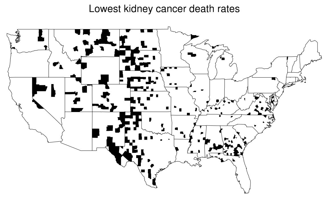
Both $\text{Figure 1}$ and $\text{Figure 2}$ show that the Great Plains has both the highest and lowest rates. Recall that the reason of this issue is sample size. Great Plains has many low-population counties; therefore rare cancer death rates, such as kidney cancer, are represented in both maps. There is no evidence from both maps that cancer rates are high (please read page 47 of the excellent book for more details).

This misleading patterns in the maps of raw death rates suggest that a Poisson model-based approach to estimating the true underlying rates might be helpful. Let’s construct a likelihood from a Poisson distribution.

$$\begin{equation} y_j \mid \theta_j \sim \text{Poisson}(10 \, n_j \, \theta_j) \tag{1}\label{eq:likelihood} \end{equation}$$

with $y_j$ denotes the number of kidney cancer deaths in county $j$ from 1980-1989, $n_j$ is the population of the county, and $\theta_j$ is the underlying rate in units of deaths per person per year.

The conjugate prior for Poisson model is Gamma distribution with parameters $\alpha$ and $\beta$:

$$\begin{equation} \theta_j \sim \text{Gamma}(\alpha, \beta). \tag{2}\label{eq:prior} \end{equation}$$

By multiplying Equation $\eqref{eq:likelihood}$ and $\eqref{eq:prior}$, we obtain the posterior

$$\begin{equation} \theta_j \mid y_j \sim \text{Gamma}(\alpha + y_j, \beta + 10 \, n_j). \tag{3}\label{eq:posterior} \end{equation}$$

Recall that the Bayes Rule states that

$$\begin{equation} \Pr( \theta_j \mid y_j ) = \frac{\Pr( y_j \mid \theta_j ) \Pr(\theta_j)}{\Pr(y_j)} \Longleftrightarrow \Pr(y_j) = \frac{\Pr( y_j \mid \theta_j ) \Pr(\theta_j)}{\Pr( \theta_j \mid y_j )}. \tag{4}\label{eq:bayes-rule} \end{equation}$$

Specifically, we will derive the predictive distribution, the marginal distribution of $y_j$, averaging over the prior distribution of $\theta_j$ or, in short, $\pmb{\Pr(y_j)}$. The objective of this post is showing this derivation.

How do we derive $\Pr(y_j)$?

Firstly, we have the likelihood, a Poisson distribution, as shown in Equation $\eqref{eq:likelihood}$

$$\begin{equation} \Pr(y_j \mid \theta_j) = \frac{1}{y_j!} (10 n_j \theta_j)^{y_j} \, e^{-10 n_j \theta_j}. \tag{5}\label{eq:likelihood-poisson} \end{equation}$$

Secondly, we also have the prior, a Gamma distribution, as described in Equation $\eqref{eq:prior}$

$$\begin{equation} \Pr(\theta_j) = \frac{\beta^\alpha}{\Gamma (\alpha) } \theta_j^{\alpha - 1} e^{-\beta \theta_j}. \tag{6}\label{eq:prior-gamma} \end{equation}$$

Last but not least, we have our posterior distribution, a Gamma distribution, as shown in Equation $\eqref{eq:posterior}$

$$\begin{equation} \Pr( \theta_j \mid y_j ) = \frac{(\beta + 10 n_j )^{\alpha + y_j}}{\Gamma (\alpha + y_j) } \theta_j^{\alpha + y_j -1} e^{-(\beta + 10 n_j) \theta_j}. \tag{7}\label{eq:posterior-gamma} \end{equation}$$

Let’s substitute Equation $\eqref{eq:likelihood-poisson}$, $\eqref{eq:prior-gamma}$, and $\eqref{eq:posterior-gamma}$ into Equation $\eqref{eq:bayes-rule}$ as follows:

$$\require{cancel} \begin{align} \Pr(y_j) &= \frac{\frac{1}{y_j!} (10 n_j \theta_j)^{y_j} \, e^{-10 n_j \theta_j} \times \frac{\beta^\alpha}{\Gamma (\alpha) } \theta_j^{\alpha - 1} e^{-\beta \theta_j} }{\frac{(\beta + 10 n_j )^{\alpha + y_j}}{\Gamma (\alpha + y_j) } \theta_j^{\alpha + y_j -1} e^{-(\beta + 10 n_j) \theta_j}} \tag{8}\label{eq:derivation-1}\\ &= \frac{1}{y_j !} \frac{(10 n_j)^{y_j} \theta_j^{y_j} e^{-10 n_j \theta_j} \frac{\beta^\alpha}{\Gamma (\alpha)} \theta_j^{\alpha-1} e^{-\beta \theta_j} \Gamma (\alpha + y_j)}{(\beta + 10 n_j)^{\alpha+y_j} \theta_j^{y_j} \theta_j^{\alpha-1} e^{-\beta \theta_j} e^{-10 n_j \theta_j}} \tag{9}\label{eq:derivation-2} \\ &= \frac{1}{y_j !} \frac{(10 n_j)^{y_j} \cancel{\theta_j^{y_j}} \cancel{e^{-10 n_j \theta_j}} \frac{\beta^\alpha}{\Gamma (\alpha)} \cancel{\theta_j^{\alpha-1}} \cancel{e^{-\beta \theta_j}} \Gamma (\alpha + y_j)}{(\beta + 10 n_j)^{\alpha+y_j} \cancel{\theta_j^{y_j}} \cancel{\theta_j^{\alpha-1}} \cancel{e^{-\beta \theta_j}} \cancel{e^{-10 n_j \theta_j}}} \tag{10}\label{eq:derivation-3} \\ &= \frac{1}{y_j !} \frac{(10 n_j)^{y_j} \beta^{\alpha} \Gamma(\alpha + y_j)}{\Gamma(\alpha) (\beta + 10 n_j)^{\alpha + y_j}} \tag{11}\label{eq:derivation-4} \\ &= \frac{1}{y_j !} \frac{\Gamma(\alpha + y_j)}{\Gamma(\alpha)} \frac{(10 n_j)^{y_j}}{(\beta + 10 n_j )^{\alpha + y_j} } \beta^{\alpha} \tag{12}\label{eq:derivation-5} \\ &= \frac{1}{y_j !} \frac{\Gamma(\alpha + y_j)}{\Gamma(\alpha)} \frac{(10 n_j)^{y_j}}{(\beta + 10 n_j )^{y_j} } \frac{\beta^{\alpha}}{(\beta+10 n_j)^{\alpha}} \tag{13}\label{eq:derivation-6} \\ &= \frac{1}{y_j !} \frac{(\alpha + y_j - 1)!}{(\alpha - 1)!} \frac{(10 n_j)^{y_j}}{(\beta + 10 n_j )^{y_j} } \frac{\beta^{\alpha}}{(\beta+10 n_j)^{\alpha}} && \text{because }\Gamma(n) = (n-1)! \tag{14}\label{eq:derivation-7} \\ &= \binom{\alpha + y_j - 1}{\alpha - 1} \left( \frac{\beta}{\beta + 10 n_j} \right)^\alpha \left( \frac{10 n_j}{\beta + 10 n_j} \right)^{y_j} && \text{because }\binom{n}{r} = \frac{n!}{r! \, (n-r)!} \tag{15}\label{eq:derivation-8} \\ &= \binom{y_j + \alpha - 1}{\alpha - 1} \left( \frac{\frac{\beta}{10 n_j}}{ \frac{\beta}{10 n_j} + 1} \right)^\alpha \left( \frac{1}{\frac{\beta}{10 n_j } + 1 } \right)^{y_j} \tag{16}\label{eq:derivation-9} \end{align}$$

As we know that a negative binomial distribution, $\text{Neg-bin}(\alpha, \beta)$, is

$$\begin{equation} \theta \sim \binom{\theta + \alpha - 1}{\alpha - 1} \left( \frac{\beta}{\beta+1} \right)^\alpha \left( \frac{1}{\beta + 1} \right)^\theta, \qquad \theta = 0, 1, 2, \ldots \tag{17}\label{eq:derivation-10} \end{equation}$$

Therefore, we conclude that $\Pr(y_j)$ in Equation $\eqref{eq:derivation-9}$ is indeed a negative binomial distribution,

$$\begin{equation} y_j \sim \text{Neg-bin}\left( \alpha, \frac{\beta}{10 n_j} \right) \tag{18}\label{eq:final-derivation} \end{equation}$$

as explained on page 49 of the book.