This article summarizes the topic “Exponentially Weighted Moving Averages” (Week 2 of Improving Deep Neural Networks: Hyperparameters tuning, Regularization and Optimization) from deeplearning.ai.

There are a few optimization algorithms which are faster than gradient descent. In order to understand these optimization algorithms, we need to understand the concept of exponentially weighted moving averages.

$\pmb{\text{Figure 1}}$: A plot of temperatures for each day in a year. Image taken from Deeplearning.ai, some rights reserved.

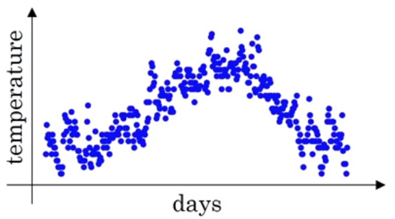
Suppose that the temperature of day $i$ is denoted by $\theta_i$ from $i=1, \ldots, 365$ (how many days in one year?). Visually, the temperatures are shown in $\text{Figure 1}$. Furthermore, we show several examples of the temperatures as follows:

$$\begin{align} \theta_1 &= 40^{\circ} \text{F} \\ \theta_2 &= 49^{\circ} \text{F} \\ \theta_3 &= 40^{\circ} \text{F} \\ &\vdots \\ \theta_{180} &= 60^{\circ} \text{F} \\ \theta_{181} &= 56^{\circ} \text{F} \\ &\vdots \end{align}$$

As we can see in the image above, the values of temperatures during a year are noisy which means that there is considerable variation in the values. The variation is caused by noise and we need to remove the variation if we want to expose the underlying values of temperatures (Brownlee, 2019).

How do we remove the noise which resides in the values of time series?

One of the techniques to remove the noise is called smoothing. Particularly, the common technique used commonly in time series forecasting is exponentially weighted averages. Computing exponentially weighted averages involves constructing a new series whose values are calculated by the average of raw observations in the original time series. Let’s denote the new series as $v_t$ for $t=1, 2, \ldots, 365$ as follows:

$$\begin{equation} v_t = \beta v_{t-1} + (1-\beta) \theta_t \tag{1}\label{eq:weighted-averages}. \end{equation}$$

with $v_t$ is the average at time $t$, $\theta_t$ is the temperature at time $t$, and $\beta$ is the parameter determining average number of days’ temperatures ($0 < \beta < 1$). Specifically,

$$\begin{equation} v_t \approx \pmb{\text{average }} \text{over } \frac{1}{1-\beta} \text{ days' temperature} \tag{2}\label{eq:parameter-beta}. \end{equation}$$

For example, let’s define $\beta = 0.9$ which means that we compute $v_t$ as approximately an average over

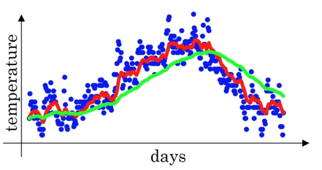
$$\begin{align} \frac{1}{1-\beta} &= \frac{1}{1-0.9} \\ &= \frac{1}{0.1} \\ &= 10 \text{ days}. \end{align}$$

Similarly, $\beta = 0.98$ gives approximately an average over $50 \text{ days}$. $\text{Figure 2}$ shows the plot of these weighted averages.

$\pmb{\text{Figure 2}}$: A plot of $v_t$ at $\beta=0.9$ ($\pmb{\text{red}}$) and $\beta=0.98$ ($\pmb{\text{green}}$). Image taken from Deeplearning.ai, some rights reserved.

As an extreme example, $\beta = 0.5$ computes approximately an average over $2 \text{ days}$ as depicted in $\text{Figure 3}$. These weighted averages are noisy because the computation of these averages takes only $2 \text{ days}$ before.

$\pmb{\text{Figure 3}}$: A plot of $v_t$ at $\beta=0.5$ ($\pmb{\text{yellow}}$). Image taken from Deeplearning.ai, some rights reserved.

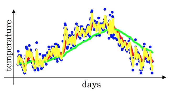
From those three different values of $\beta$, we can see that as $\beta$ is getting larger and larger, the plot is going smoother and smoother. On the other hand, if $\beta$ is getting smaller and smaller, the plot will become noisier and noisier. As a conclusion,

$\begin{align} \beta \ggg \; &\Longrightarrow \pmb{ \text{ smoother}} \text{ because we are averaging more days} \\ \beta \lll \; &\Longrightarrow \pmb{ \text{ noisier}} \text{ because we are averaging fewer days}. \end{align}$

Bias Correction

Previously, we have defined Equation $\eqref{eq:weighted-averages}$ which is

$$\begin{equation} v_t = \beta v_{t-1} + (1-\beta) \theta_t. \end{equation}$$

Let’s substitute $v_{0} = 0$ and $\beta = 0.98$ into Equation $\eqref{eq:weighted-averages}$.
At $t=1$,

$$\begin{align} v_1 = \beta v_{0} + (1-\beta) \theta_1 &\Leftrightarrow v_1 = (0.98) (0) + (1-0.98) \theta_1 \\ &\Leftrightarrow v_1 = 0.02 \; \theta_1 \tag{3} \label{eq:v-1}. \end{align}$$

At $t=2$,

$$\begin{align} v_2 = \beta v_{1} + (1-\beta) \theta_2 &\Leftrightarrow v_2 = (0.98) (0.02 \; \theta_1) + (1-0.98) \theta_2 \\ &\Leftrightarrow v_2 = 0.0196 \; \theta_1 + 0.02 \; \theta_2 \tag{4} \label{eq:v-2}. \end{align}$$

With the assumption that $\theta_1$, $\theta_2 > 0$, we arrive at

$$\begin{equation} v_2 \ll \theta_1 \text{ and } v_2 \ll \theta_2 \end{equation}$$

which means that $v_2$ is not a very good estimate of the first two days’ temperature of the year.

How can we improve the estimate of the first two days’ temperature?

Introducing bias correction will improve the estimate. With $\beta = 0.98$,

$$\begin{align} v_t &\approx \text{ average over } \frac{1}{1-0.98} \\ &\approx \text{ average over } 50 \text{ days' temperature}; \end{align}$$

moreover, at $t=2$, the bias correction factor will be

$\begin{align} 1 - \beta^t &= 1 - (0.98)^2 \\ &= 0.0396 \tag{5} \label{eq:bias-correction} \end{align}$ Therefore, the bias correction for $v_2$ will be

$$\begin{align} \frac{v_2}{1-\beta^2} &= \frac{v_2}{0.0396} & \text{ from Equation }\eqref{eq:bias-correction}. \end{align}$$

Since $v_2$ is divided by $0.0396$ which acts as a bias correction, the bias from $v_2$ will be removed and the estimate of $v_2$ is improving. Generally, the form of weighted averages with bias correction is defined as

$\begin{equation} \frac{v_t}{1 - \beta^t} = \beta \; v_{t-1} + (1 - \beta) \; \theta_t. \tag{6} \label{eq:with-bias-correction} \end{equation}$ with $t=1,2, \ldots, 365$.

As a final note, the bias correction helps us find better estimates of a series during the initial phase of learning as we will see in the Part 2 of this blog. As $t$ is getting larger and larger, $\beta^t \approx 0$. Therefore, if $t$ is large, the bias correction will have no effect on the series.

References

Brownlee, J. (2019). Introduction to Time Series Forecasting in Python. https://machinelearningmastery.com/introduction-to-time-series-forecasting-with-python/. Accessed: 2020-09-5