
This article explains forward propagation and backpropagation for one data instance in one round.
Suppose that we have an artificial neural network (ANN) for doing binary classification which consists of one hidden layer. Particularly, the hidden layer has 3 nodes or units with each has a sigmoid activation function ($\sigma$) as shown in the image below:
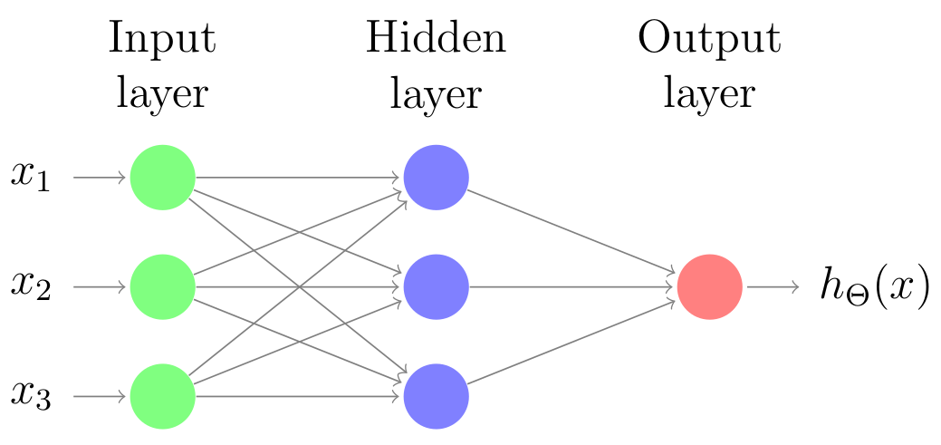
Concretely, the input and hidden layer also have a bias unit respectively (not shown in the image). We stick to Andrew’s notation from his excellent Machine Learning Coursera. Let’s define our data instance
\[\begin{equation} x = \begin{bmatrix} 1 \\ x_1 \\ x_2 \\ x_3 \end{bmatrix}.\tag{1}\label{eq:data-instance} \end{equation}\]Our ANN also has the true label, $y$ and two weight matrices, $\Theta^{(1)}$ and $\Theta^{(2)}$ specified as follows: \(\begin{align} \Theta^{(1)} &= \begin{bmatrix} \Theta_{10}^{(1)} & \Theta_{11}^{(1)} & \Theta_{12}^{(1)} & \Theta_{13}^{(1)} \\ \Theta_{20}^{(1)} & \Theta_{21}^{(1)} & \Theta_{22}^{(1)} & \Theta_{23}^{(1)} \\ \Theta_{30}^{(1)} & \Theta_{31}^{(1)} & \Theta_{32}^{(1)} & \Theta_{33}^{(1)} \end{bmatrix} \text{ and} \tag{2}\label{eq:weight-matrix-1} \\ \Theta^{(2)} &= \begin{bmatrix} \Theta_{10}^{(2)} & \Theta_{11}^{(2)} & \Theta_{12}^{(2)} & \Theta_{13}^{(2)} \end{bmatrix}. \tag{3}\label{eq:weight-matrix-2} \end{align}\)
Now firstly, let us compute for forward propagation. Here is the computation for the hidden layer.
\[\begin{align} \underbrace{z^{(2)}}_{3 \times 1} &= \underbrace{\Theta^{(1)}}_{3 \times 4} \underbrace{x}_{4 \times 1} \tag{4}\label{eq:z-2} \\ a^{(2)} &= \sigma(z^{(2)}) \tag{5}\label{eq:a-2} \\ a^{(2)} &= \begin{bmatrix} 1 \\ a_1^{(2)} \\ a_2^{(2)} \\ a_3^{(2)} \end{bmatrix} & \text{add a bias unit.} \tag{6}\label{eq:a-2-bias} \end{align}\]Now we compute the output layer as follows:
\[\begin{align} \underbrace{z^{(3)}}_{1 \times 1} &= \underbrace{\Theta^{(2)}}_{1 \times 4} \underbrace{a^{(2)}}_{4 \times 1} \tag{7}\label{eq:z-3} \\ a^{(3)} &= \sigma(z^{(3)}) \tag{8}\label{eq:a-3} \\ h_\Theta(x) &= a^{(3)}. \tag{9}\label{eq:h-x} \end{align}\]We have finished our forward propagation. Basically, forward propagation computes our model’s prediction. Now let us compute the backpropagation steps. Backpropagation algorithm calculates gradients; subsequently, the gradients are needed to update our weight matrices. Consequently, the updates should make our model’s current prediction better than the previous one.
Here is the backpropagation steps.
\[\begin{align} \underbrace{\delta^{(3)}}_{1 \times 1} &= \underbrace{a^{(3)}}_{1 \times 1} - \underbrace{y}_{1 \times 1} \tag{10}\label{eq:delta-3} \\ \underbrace{\delta^{(2)}}_{4 \times 1} &= \underbrace{(\Theta^{(2)})^T}_{4 \times 1} \underbrace{\delta^{(3)}}_{1 \times 1} \odot \underbrace{a^{(2)}}_{4 \times 1} \odot \underbrace{(1 - a^{(2)})}_{4 \times 1} & \odot = \text{element-wise multiplication} \tag{11}\label{eq:delta-2} \\ \delta^{(2)} &= \begin{bmatrix} \delta_1^{(2)} \\ \delta_2^{(2)} \\ \delta_3^{(2)} \end{bmatrix} & \text{remove }\delta_0^{(2)}. \tag{12}\label{eq:delta-2-remove-bias} \end{align}\]We have completed our backpropagation algorithm.
Finally we can update our weight matrices as follows: